Activation Functions

Neuron Model

The operation of a neuron in an artificial neural network is, to sum up, the product of the input and associated weight (also called connection weight) and produce an output using activation/transfer function. It maps the output values in the desired range such as 0 to 1 or -1 to 1 or 0 to inf. This output will act as an input for neuron of next layer.

For input x0, connection weight is w0. Inside the cell, the first half is responsible for summation of the product of input and associated weight and second half is applying a transfer/activation function on that summation.

There is no activation at the input unit of a neuron or we can say it is identity function (f(x) = x).

All the neuron of a particular layer gets the same activation functions. Different layers can have different activation function. For example: In a classification network generally, there is a sigmoid/ReLU activation in intermediate layers and softmax at the output layer.

Why do we need activation functions?

The one line answer is “To add non-linearity”.

We want out Neural Networks to be a Universal Function Approximators. It means we can compute and learn any complex function which maps inputs to outputs. If we do not apply a Non-linear Activation function, the final output would simply be a simple linear function. It cannot learn function mapping from complex and high dimensional data like images, videos, speech etc. Non-linear function is needed for the Universal Function Approximators. 

The Universal Approximator theorem states that under certain conditions, for any continuous function f:[0,1]^d→R and any ϵ, there exist a neural network with one hidden layer and a sufficiently large number of hidden units m which approximates f on [0,1]^d uniformly to within ϵ. One of the conditions for the universal approximation theorem to be valid is that the neural network is a composition of nonlinear activation functions: if only linear functions are used, the theorem is not valid anymore.

What if we add more layers without using any Non-Linear Function?

A neural network with linear activation functions and n layers each having some m hidden units is equivalent to a linear network without any hidden layers because the composition of any number of linear functions is a linear function only, It can be proved using below equation.

Y =h(x)

= b_{n +}W_n (b_n-1 + W_n-1(…(b₁+W₁x)…))

=b_n+W_nb_n-1+W_nW_n-1b_n-1+…+W_nW_n-1…W₁x

= b¹+W¹x 

Hence adding more layers (“going deep”) doesn’t help for a linear neural network at all, unlike nonlinear neural network.

Therefore, we need to apply a non-linear Activation function to make the network more powerful to represent non-linear complex functional mapping function between input and output for any data.

Commonly used Activation Functions:

Sigmoid

• f(x) = 1/ (1+exp(-x) ) 
• It squashes the input in the range [0,1].
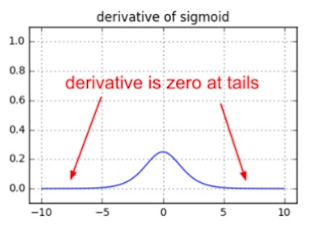
• Derivative: z(1-z)
• Historically popular since they have nice interpretation as a saturating firing rate of a neuron.
• exp is a bit compute expensive.
• Saturated neuron kills gradient.
• Sigmoid output is not zero centered.
• slow convergence.
• Vanishing Gradient Problem.

Hyperbolic tangent Function tanh(x)

tanh(x)

• Squashes input to range [-1, 1]
• Derivative: z(1-z²)
• Zero Centered
• exp is a bit compute expensive.
• Saturated neuron kills gradient.

Rectified Linear Unit (ReLU)

• f(x) = max(0, x) 
• Derivative : 1, if x> 0 else 0 
• Range [0, inf ]
• Does not saturate ( in + region)
• Computationally very efficient
• Converges much faster than sigmoid/tanh
• Not Zero Centered
• Neuron Dies sometimes

Leaky ReLU

• f(x) = max(0.01x ,x)
• All benefit of ReLU
• Will not Die
• Parametric ReLU : max(ax,x) , a can be variable

Quick Summary 

• Use ReLU, but be careful about your learning rate.
• Try Out Leaky ReLU/ELU
• You can try tanh but don't expect much.
• Don't use sigmoid in intermediate layers.